Tutorial 10: Simulation cell relaxation
- Author:
Chris-Kriton Skylaris
- Date:
August 2023
Introduction
This tutorial demonstrates how to use ONETEP to relax the simulation cell of a crystalline material
Cell relaxation of bulk crystalline silica
This calculation will relax the lattice of a silica (SiO2) simulation cell, which is depicted below:
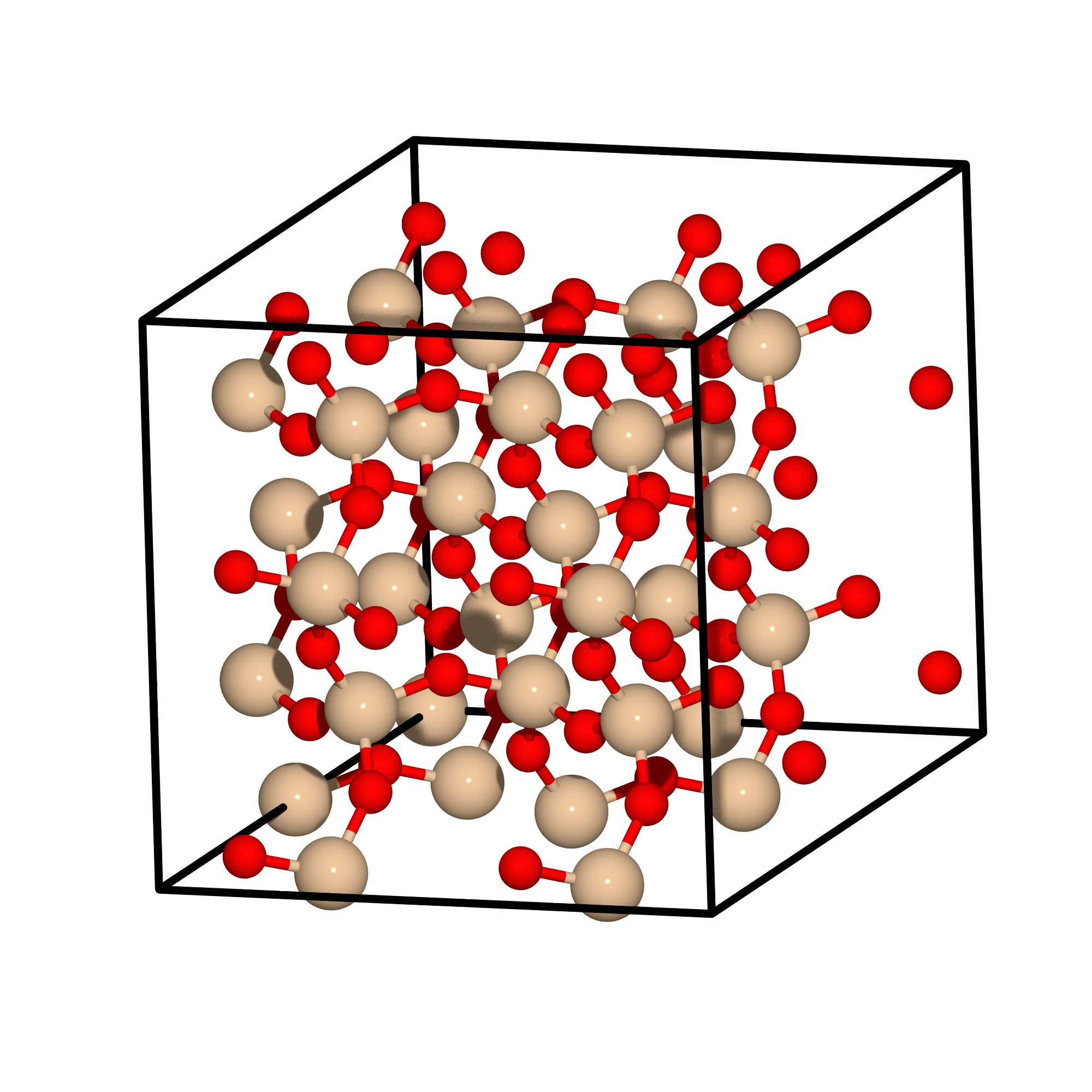
Fig. 9 The simulation cell of silica.
The simulation cell of silica used in this tutorial. The silicon atoms are colored beige and the oxygen atoms are colored red.
Input file keywords
The input file, which is provided, is called silica96.dat and contains
96 atoms in total.
To perform cell relaxation the
task STRESS
keyword is required.
You will notice in the input file also the following keywords related to the cell relaxation:
stress_tensor T
stress_elasticity F
stress_relax T
stress_assumed_symmetry tetra1
stress_relax_atoms T
Where stress_tensor T instructs the code to compute the stress tensor,
while the calculation of elestic constants is trned off with
stress_elasticity F.
In this calculation the simulation cell will be relaxed (in order to determine
the optimal lattice vectors) and this is denoted by stress_relax T.
In this calculation, in addition to the simulation cell we want do relax also
the coordinates of the atoms and for this we use the keyword
stress_relax_atoms T.
It is worth noting here that the atomic coordinates would also be relaxed if the
stress_relax_atoms was set to F (False), but in this case they
would only be “stretched” to be commensurate with the change in the lattice
vectors, in other words they would retain the same fractional coordinates.
On the other hand if the stress_relax_atoms is activated the coordinates
of the atoms are fully relaxed and are not comstrained to remain equal to the
fractional coordinates they had at the start of the calculation.
Finally the stress_assumed_symmetry tetra1 instructs the code to assume
a particular symmetry for the simulation cell and maintain this symmetry during
the cell relaxation.
Is the symmetry of the cell is known and is supported by the code (see the user
manual) is is important to activate it with this keyword as it will
significantly reduce the number of single point energy calculations that will be
performed.
Running the calculation
Now run the calculation and examine the output. Lets examine the output step by step noting the various stages of the calculation.
At the very beginning some information about the initialisation of the calculation is produced such as:
PSINC grid sizes: information about the grids used for the psinc basis functionsAtom SCF Calculation for...: here the code initialises the NGWFs with atomic orbitals created specificaly for the valence electrons of the chosen pseudopotentials and confined within the NGWF spherical regions.STRESS: undistorted cell: this is the beginning of the very first energy calculation from which calculations with applied stains will be subtracted to compute the stress tensor.Atomic positions optimised prior to stress calculation: a geometry relaxation is performed first since we have specifiedstress_relax_atoms T.
You will notice that this calculation takes 30 NGWF iterations to converge as a
very tight convergence criterion for the NGWFs
(ngwf_threshold_orig 1.e-7) has been applied in the input.
This was done to ensure very accurate forces and it may be a bit extreme, but it
is better to be on the safe side.
After this energy evaluation the code computes the forces and compares them with
the threshold that has been defined for geoemetry relaxation.
In this calculation you will notice that the forces are small and below the
tolerance (|F|max 1.e-3 Eh/Bohr) that has been set for the convergence
of the geometry.
As a result the code reports that the geoemetry relaxation has been completed
with the message “Geometry optimization completed successfully”.
Calculation of the stress tensor
Then the calculation proceeds to evaluate the energy of the system at different
distortions (strains) of the lattice vectors in order to compute the stress
tensor.
The beginning of this procedure is denoted by the
STRESS: distorted cells message.
The stress tensor computed is summarised at the end of the first iteration of cell relaxation:
stress_tensor: iteration 1
This stress tensor is now used to change the simulation cell. Again a geometry relaxation is performed which converges at the first step. Then several single point energy calculations follow to compute a new stress tensor until we obtain the summary of the second iteration:
stress_tensor: iteration 2
Finally, we see that in the third iteration the cell has been relaxed. The relaxed cell is printed:
Relaxed cell:
  bohr
19.07668106      0.00000000      0.00000000
 0.00000000     19.07668106      0.00000000
 0.00000000      0.00000000     27.83315074
This completes tutorial 10.
Files for this tutorial: